Thursday, December 18, 2014

Experiments with the RFM69 433MHz digital transceiver module

Summary: 

This post is an overview of an board I'm developing which encapsulates the RFM69 radio module with a MCU to expose a simple UART API which can be tailored for specific applications. This simplifies embedding a radio into existing applications with very little additional expense in terms of hardware or power budget. The API is implemented by a light weight radio OS (currently just 5KiB) which is open source and the bill-of-materials for the board can be as little as $8 / €7.

Background to project:

WRSC2014 contestant Team FASt from University of Porto.
The World Robotic Sailing Championship 2014 was held in Galway Ireland (my home town) in September this year. It was originally anticipated that each contestant would use a RFM69 radio module to relay real time positioning information back to a central hub for recording the race and scoring. It was also hoped that the race organizers could use the same radio network to broadcast race waypoints, starting times, obstacles etc. However given the short time available it became clear that race contestants would not have sufficient time to incorporate this module into their hardware and write the associated supporting firmware.

Based on the experience of WRSC 2014 I believe the best solution for such competitions is to develop a low cost ready made 'black box' which is given (ready made and programmed) to each contestant. The black box would expose a very simple API to the boat's software which should not take long to integrate. Or if it's a case the contestant simply does not have time to make any changes to their software the radio can be mated with a GPS module and it will send real time position, speed and heading back to the race organizers.

This project is the first step in such a system.  An entire race system will incorporate other elements such as base station software, real time visualization tools, race protocols etc. This blog post only discusses the radio board.

RFM69 family of modules:

The RFM range of modules are made by HopeRF and based on the Semtech radio ICs. The RFM69 comes in several varieties. The one I've been using is the higher power version: the RFM69HW [1] which is based on the Semtech SX1231H [2]  chip.

Feature highlights:
  • Digital SPI interface
  • Operates on 433MHz unlicensed ISM band
  • Continuous or packet mode (66 byte FIFO)
  • Built in AES encryption and CRC-16 engine
  • Configurable bit rates up to 300kbps
  • Configurable power settings
  • Line-of-sight ranges in excess of 1km
  • Sleep current < 1µA
  • Only $4 in small quantities

The radio board:

This is the general architecture of the board: a MCU acts as the go between the application hardware and software and the RFM69 radio module. The MCU takes care of all the complex register configuration of the RFM69 and takes of low level functions (such as responding to pings, remote configuration commands etc) without ever bothering the application. The application talks to the MCU thru a standard UART interface using a very simple protocol.
In addition to the core API there is also the option to compile in application specific functions (for example I've build in support for a rain tip-bucket and a temperature sensor: more on that later).


Prototype mk1:

Unfortunately these modules have a 2mm pad pitch making them difficult to use directly with standard 2.54mm spacing prototype board or breadboard. So for the first prototype I glued the module onto a prototype board and used thin 30AWG wire to link the module pads to pads on the protoboard.


Reasonably need looking from above...


The problem is on the underside...


Even though it's only a hand full of wires, cutting, stripping and soldering these is very time consuming and error prone (well in excess of three hours per board).

For the first prototype I used a LPC810 ARM Cortex-M0+ MCU as the controller.  The ARM Cortex-M range is my MCU of preference these days due to the ease of 32 bit programming, open source and well supported tools and a wide range of vendors (NXP, TI, Freescale etc).

This 8 pin DIP, 4KiB program memory device was adequate for initial tests, but I quickly ran up against the 4KiB program limit. The 8 pin DIP package also had the advantage that I could socket it and try different versions of firmware just by swapping out the device.

With two of these modules I did some range tests. I soldered 17cm wire (quarter wave at 433MHz) to both sides of the board just at the RFM69 antenna output pad. I was able to achieve two way communication of about 1km along the (line-of-sight) length of the Doughiska Road in east Galway city.


Prototype mk2:

For the next prototype I moved to the LPC812: in many ways identical to the LPC810 but with more IO pins and more memory (16KiB program memory, 4KiB SRAM). Rather than use time consuming protoboard I decided it was worth spending some money on a PCB. I designed a two layer board using the free version of CadSoft Eagle and used Eurocircuit's standard FR4 pool to fabricate. This job cost €80, but for that I got 20 boards. The turn around time was nominally 10 working days, but I had them in a week.


The board in the photo actually comprises two boards:  one for the RFM69 discussed here and another for a similar (better?) module the RFM98 which I'll discuss in another blog post. The two halves are separated with a hacksaw.

One very handy feature of the LPC81x range of MCU is the switch matrix which allows many of the MCU functions to be mapped to an arbitrary pin.  This makes PCB layout a lot easier.

After populating with the MCU, module and 3 other components (LED, resistor and decoupling capacitor for MCU) this is what the board looks like. There is the option to use a wire as antenna, or alternatively splash out on a SMA connector (probably the most expensive component on the board!). This photo shows a SMA connector with a 433MHz stub antenna obtained from Farnell [3].


On the left is the UART connector for the radio API, pins for Serial Wire Debug (SWD) for debugging and reprogramming. Left top is the power connector (3.3V nominal, but will work down to 1.8V).

There is also a LED at the very top-left. This is a general purpose indicator that's under control of the MCU. I use this to flash a sequence after boot up tests are complete and flash it each time a packet is sent or received.

In the center there is an option for another connector which will give direct access to the RFM69 SPI port for debugging, or simply using the PCB as a breakout board for the radio module (leaving the MCU pads unpopulated).

The bill of materials is PCB €2;  LPC812M101JD20 €1.50; RFM69HW €3 ; passives, pin headers €0.50; SMA connector (optional) €3.50 ; stub antenna (optional) €5. That's a total of €7 without the SMA connector option. Those prices with the exception of the PCB are for single quantities from Element 14's catalog.  Significant discounts are usually available when ordering 20+. Also components can often be sourced at a much lower cost from Chinese retailers (eg Alibaba and Deal Extreme). The PCB cost is more complex: many fabricators have a fixed job charge (it was about €50 for Eurocircuits) and they then charge per PCB after that. So if you make a lot of them the price per board goes down quickly. If you make just one it will be very expensive.


The radio OS firmware:

My firmware is written in C and currently uses the LPCXpresso IDE to build. This uses the GCC compiler under the hood. The main purpose of the firmware is to expose an simple UART API which the host application uses. The API protocol is simple: a single character command/response code followed by parameters separated by spaces followed by a carriage-return to end the command. All parameters are in hexadecimal. Example:

application to radio:
T 44 5232

'T' means transmit a packet. It takes two parameters: the to-address and the packet payload.

radio to application:
p FF 42 7A14051F003D AD

The 'p' response code is transmitted to the application whenever a packet is received. There are four parameters: the to-address (FF hex being the broadcast address),  from-address, the packet payload and the RSSI (received signal strength indicator). 

Other commands include 'R' and 'W' to read/write RFM69 radio configuration registers. 'M' to switch operating mode from an active awake/listening (20mA current use) to a sleep-polling mode using an average of about 140µA.

Some advanced experimental commands are remote register read/write, allowing a remote radio to be reconfigured. Remote watchdog timer configuration which will reset the radio to default configuration should there be a prolonged loss of communication. Remote command execution (which can be used for remote configuration and to relay packets), remote battery voltage measurement.


Test application:

As mentioned earlier the intended application is for robot sailboat telemetry. But I'm conducting initial tests by using one of these radios with a rain tip-bucket and temperature sensor in my garden. I've got the radio board in an IP66 enclosure with a small PV panel and LiPo battery (and associated charger). 

The tip-bucket causes a magnet to fly past a reed-switch each time the bucket tips. I use this in conjunction with one of the spare LPC812 pins and an interrupt channel to count each time this happens. I've also got a DS18B20 temperature sensor on another spare pin. 

I run this in low power polling mode. Every 30 seconds the MCU comes out of deep sleep mode, makes a temperature measurement and fires up the transmitter and sends a status packet with the tip bucket counter, current temperature, and battery voltage [4]. It listens for about 100ms for a response packet. If none is received it goes back into deep sleep mode. 

If I need to communicate to the out door unit I must wait for a poll packet and then immediately send my command. If multiple commands need to be issued, the first command is to switch the radio into active listen mode, issue all the necessary commands and then put back into low power mode.

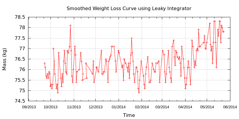
So far tests have been successful with the only communications disruptions attributed to either running out of battery charge (it's winter here and the days are short: unless  it's a sunny day there is not enough stored charge to keep it going through the night) or a problem with the USB/Serial cable at the receiving end.

This is 48 hours of some sample data. The disruptions are due to problems with the USB/Serial cable at the receiving end: the radio worked flawlessly. Also note the elevated temperatures are due to the sun falling directly on the IP66 box. 


Current and future work:

I'm currently working an a web browser based application/UI to interact with these radios. The application will allow configuration of the local and remote radios, performing experiments with various radio settings. Monitoring network performance etc.

Also I'm planning to make a third prototype. This will be smaller than the current board, perhaps putting the MCU on the underside of the board. I'm also considering moving to the recently announced LPC82x MCUs [ref] which feature more program flash, more SRAM, a full ADC and other new features.

Features for future firmware include mesh networking, encryption, remote program execution and over-the-air firmware upgrades.


Conclusions:

So far I'm very impressed with these radio modules. At only $4 they're a steal. I've verified two way communication at over 1km distance line-of-sight and I've heard reports of success well in excess of 1.5km line-of-sight. With the addition of an LPC812 MCU with my radio OS and simple UART API, embedding this radio into an application is far simpler than building the radio driver directly into the application software. The entire bill of materials is about $7 with the option of a SMA connector which might bring it to $10. My PCB layout is available under the BSD licence on GitHub [5] and the firmware is also available on GitHub [6].


Footnotes:

[1] RFM69 Datasheet
http://www.hoperf.cn/upload/rf/RFM69-V1.3.pdf

[2] Semtech SX1231H product information and datasheet
http://www.semtech.com/wireless-rf/rf-transceivers/sx1231h/

[3] Farnell/Element 14 SKU 2305893, €4.86 in single quantities.

[4] One feature I miss in the LPC81x range of MCU is a full ADC. There is however a comparitor which can be used with a voltage ladder to make crude voltage measurements. I use this for battery voltage measurement (Vcc thru voltage ladder on one comparitor input, and the built in 0.9V voltage reference on the other). In my tests it can detect low battery voltage condition, but due to the coarse resolution I get a warning only about a hour before the voltage drops below the cutoff threshold.

[5] https://github.com/jdesbonnet/RFMxx_LPC812

[6] https://github.com/jdesbonnet/RFM69_LPC812_firmware

Updates:

11 Feb 2015: Added link to firmware repository on GitHub.

Sunday, August 31, 2014

Open IC Register Description Language (a proposal)

Summary: Many modern digital ICs are interacted with through memory mapped registers. Writing maintainable code demands a header file with well structured constants for register addresses, bit field masks, field values etc. But even that on its own doesn't guarantee readable code. It is often desirable to have a summary of the register function, and values in a comment block above the code. But this can be very onerous, involving lots of cutting/pasting/formatting from the datasheet. My proposal is a standard machine-readable way to describe a ICs registers using an open format. These descriptions can be used to generate constant header files for any language, automatically document code and provide useful plugins for IDEs. I also propose to crowd-source an open source data repository of such description files for popular ICs. 
I've been writing some embedded C recently, and trying to document my code as I go along. When I access an IC register I include the following information above the code block:
  • The datasheet document name and revision number
  • The relevant section / table number/ page number in the datasheet
  • A short description of the register / bit field being accessed and allowed values
This can get quite tedious cutting/pasting text from the datasheet. Any time something is cut/paste more than twice is a strong indicator that you are doing something wrong.

I went looking for any standard machine-readable way to document IC registers and found nothing (so far). So I'm proposing an open standard and open database to document IC registers.

This will have several benefits for developers:
  • automatically generate header files for what ever language is being used with register addresses, bit masks, field values etc. Automatic generation guarantees a consistent format.
  • automatically generate data structures for large/complex registers
  • automatically document code by making a single reference to a register / bit field
  • allow tight integration with IDEs (eg debugger can display annotated register values along with the actual meaning of that value)
I'm not a big fan of XML, but it does seem to be the standard for this kind of thing. So my proposed IC register description will look something like this:

<?xml encoding="utf-8">
<device name="RFM69">

<description>
HopeRF RFM69/RFM69HW radio module
</description>

<register>
<sname>OpMode</sname>
<name>Operation Mode</name>
<address>0x01</address>

<bitfield bit="7" rwmode="rw">
<sname>SequencerOff</sname>
<description>Controls the automatic Sequencer (see section 4.2)
<value val="0"></value>
<value val="1">Mode is forced by user</value>
</bitfield>

<bitfield bit="6" rwmode="rw" type="onoff">
<sname>ListenOn</sname>
<description>Enables Listen Mode, should be enabled whilst in Standby mode.</description>
</bitfield>

<bitfield bit="4:2" rwmode="rw">
<sname>Mode</sname>
<description>Tranceiver's operating mode</description>
<reference>section 6.2</reference>
<fieldvalue><value>0</value><sname>SLEEP</sname><name>Sleep mode</name></fieldvalue>
<fieldvalue><value>1</value><sname>STDBY</sname><name>Standby mode</name></fieldvalue>
<fieldvalue><value>2</value><sname>FS</sname><name>Frequency Synthesis mode</name></fieldvalue>
<fieldvalue><value>3</value><sname>TX</sname><name>Transmitter mode</name></fieldvalue>
<fieldvalue><value>4</value><sname>RX</sname><name>Receiver mode</name></fieldvalue>
</bitfield>

</register>


<register>
<sname>DataModul</sname>
<description>Data modulation settings</description>
.... etc....
</register>

</device>


Some notes about the schema: Along with a human friendly register name, I've got a short-name. This will conform to C identifier specification and is used in header file generation.

The resulting header files can be generated from rules (which can be changed according to house style). For example my rule is: <IC>_<REG> for register address, <IC>_<REG>_<FIELD>_MASK for bit field masks, and for each field value <IC>_<REG>_<FIELD>_<FIELDVALUE>. So from the XML example above I get something like this for the C language header file:

#define RFM69_OPMODE (0x01) /* Operation mode register */
#define RFM69_OPMODE_MODE_MASK (7 <<2)
#define RFM69_OPMODE_MODE_SLEEP (0<<2) /* Sleep mode */
#define RFM69_OPMODE_MODE_STDBY (1<<2) /* Standby mode */
#define RFM69_OPMODE_MODE_FS (2<<2) /* Frequency synthesiser mode */
#define RFM69_OPMODE_MODE_TX (3<<2) /* Transmitter mode */
#define RFM69_OPMODE_MODE_RX (4<<2) /* Receiver mode */

Code documentation.

Comment annotations can instruct a code post-processor to insert/update the necessary documentation. For example:

/**
 * Set transceiver mode to transmit
 * @register RFM69_OPMODE.MODE
 */

Will get expanded to something like this:

/**
 * Set transceiver mode to receive
 *
 * @register RFM69_OPMODE.MODE
 *
 * RFM69_OPMODE.MODE autodoc. Do not edit. ****
 * RFM69 datasheet, section 6.3
 * OPMODE MODE (bits 4:2). Read and write allowed. Values:
 * SLEEP (0) : Sleep mode ;  STDBY(1) : Standby mode ;
 * FS (2): Frequency synthesis mode ; TX (4): Transmitter mode;
 * RX (4): Receiver mode
 * End RFM69_OPMODE.MODE autodoc
 */

Note the auto generated sections are delimited by a marker. While this may generate verbose source code it will be easier to read (especially for someone new to the hardware) and can be easily maintained/updated or removed as required.

This can also be helpful for non-english speaking developers. Any text element in the register description can have a lang (language) attribute. So a developer can switch out the english descriptions for one in their native language (either permanently or temporarily with an IDE plugin).

The open database:

I propose that these IC description files are uploaded and maintained on something like GitHub repositories. For ease of maintenance, it might be an idea to split the description file into a separate file for each register. A suitable licence must be used to ensure the generated header files and documentation do not cause any licencing restriction on developers.

Other features/ideas:
  • Chip variants or silicon revisions can be accommodated by linking to a root document and then including only items that have been changed.
  • IDEs can generate convenience routines eg in the example above function rfm69_mode_set (mode); rfm69_mode_get(); etc
  • IDEs can use this description to visually annotate register bit fields in the debugger
  • Complex configurations and sequences can be documented by the manufacturer in a machine-readable but language neutral way.
  • Support i18n, allowing a language attribute for any text fields.
  • Editing XML directly is tedious and error prone. A web app could be used as a front end for editing and maintaining such a database.
  • What I've proposed is only for registers, but other common information could also be included (pin outs, voltage/current ratings etc)
I've stared writing some utilities to implement some of these ideas for an internal project which I'll release as an open source project soon (probably under a BSD style licence). I'd be delighted to hear from anyone who is aware of any similar efforts (I really don't want to reinvent the wheel here), or would like to critique or contribute.

Updates:

3 Sep 2014: I've created a GitHub respository for this project at https://github.com/jdesbonnet/ICRDL

Tuesday, June 10, 2014

Weight charts from wwdiary, part 2

In part 1 [1] I described a way of generating nice weight charts from the data stored in the wwdiary [2] weight loss app.

I record a daily weight measurement, usually first thing each morning. As one would expect this can vary a lot from day to day for all sorts of reasons. To get a better handle of the trends a smoothing filter can be applied to the data. There are many methods of doing this, eg Moving Averages. The one I've opted to use here is the Leaky Integrator [3] due to its simplicity.

The unsmoothed chart looks like this.


The following is a GnuPlot chart that applies the Leaky Integrator smoothing to the data (assumed to be in file weight.dat, see part 1 on how to extract this from the wwdiary database):

# GnuPlot script to plot smoothed weight from datafile in format
# uuuuuuuuuu ww.w
# Where uuuuuuuuuu is date in unix epoch time
# and ww.w is weight (in kg here, but trivial to change to other units).
# One record per line. 
# 
# Smoothing is acomplished with the Leaky Integrator
# http://en.wikipedia.org/wiki/Leaky_integrator
# 
# Joe Desbonnet, jdesbonnet@gmail.com, June 2014.
#
set xdata time
set timefmt "%s"
set format x "%m/%Y"
set xtics font "Arial, 10" 
set title "Smoothed Weight Loss Curve using Leaky Integrator λ=0.8"
set xlabel "Time"
set ylabel "Mass (kg)"
set grid
set key off
set term pngcairo size 800,400
set output "weight.png"
# Lambda (0 ≤ λ < 1.0) determines smoothing. Higher values for more smoothing.
lambda=0.8
ym1=0
leaky_integrator(x) = (ym1 = ym1==0 ? x : (1-lambda)*x + lambda*ym1)
plot 'weight.dat' using 1:(leaky_integrator($2)) with linespoints, \
     'weight.dat' using 1:2 lt 3


After applying the smoothing filter (and plotting the original points in blue for reference):


You can adjust the 'strength' of the smoothing filter by changing the value of lambda. Lambda can vary from 0 to 1. The closer to 1 the higher the smoothing effect.

References:

[1] http://jdesbonnet.blogspot.ie/2014/06/weight-charts-from-wwdiary-part-1.html
[2] https://play.google.com/store/apps/details?id=com.canofsleep.wwdiary
[3] http://en.wikipedia.org/wiki/Leaky_integrator

Monday, June 9, 2014

Weight charts from wwdiary, part 1

I've been using an excellent Android app called wwdiary [1] for over two years to lose (and then manage) my weight. The app allows you to record your daily weight, but unfortunately has no inbuilt charting [2]. So I wrote a script to extract the data and make my own charts.

Here is my chart:

Here's how to make your own:

This recipe requires a few command line tools. I'm using Linux, but to the best of my knowledge all these tools are available for Windows and Mac and should work exactly the same way described below. You'll need SQLite (there are several implementations), and GnuPlot.

wwdiary uses the SQLite database engine for storage, and you can grab a copy by going into the app settings and saving a copy of the database to SD Card. Copy this file to your computer using whatever file transfer tools you have to hand (I often just email it to myself using the gmail app file-attach option). Let's call this file wwdiary.database.

First you need to extract the weight from the SQLite database in a format that's easy for GnuPlot to parse.  Create a SQLite script file. Let's call it extract_weight.sqlite:

.separator "\t"
select date/1000,weight*0.453592 from weightlog;
.quit

Note the "/1000" is to convert the unix epoch timestamp in milliseconds to seconds and the "*0.453592" is to convert imperial pounds used internally in the app [3] to kg. Run the script and send the output to weight.dat:

sqlite3 wwdiary.database < extract_weight.sqlite > weight.dat


The contents of weight.dat should look something like this:

1379890800 76.2999384291992
1379977200 76.0999346446533
1380063600 75.6999409180908
1380150000 75.5999355651855
...

Create the plot script, call it say weight.gp:

# GnuPlot script to plot weight in format
# uuuuuuuuuu ww.w
# Where uuuuuuuuuu is the unix epoch time in seconds
# and ww.ww is weight (I use kg, but use what you like).
# 
# Joe Desbonnet, jdesbonnet@gmail.com, June 2014.
#
set xdata time
set timefmt "%s"
set format x "%m/%Y"
set xtics font "Arial, 10" 
set title "Weight Loss Curve"
set xlabel "Time"
set ylabel "Mass (kg)"
set grid
set key off
set term pngcairo size 800,400
set output "weight.png"
plot 'weight.dat' using 1:2 with linespoints


And now run it:

gnuplot weight.gp

All going well, you should find a PNG image file called weight.png in the same folder with your weight chart.

In part 2 I'll show you how to apply a smoothing filter to the chart.

References

[1] https://play.google.com/store/apps/details?id=com.canofsleep.wwdiary
[2] There is a subscription service available where a chart can be viewed on an online dashboard.
[3] Oh please if you're designing software use SI (metric) units under the hood. Convert to antiquated Olde Worlde/American units at the user interface if you must. Even the Apollo moon avionics software from 1960s USA calculated in SI, converting to feet, furlongs, hundred-weight etc only at the last second at the user interface. (See http://dodlithr.blogspot.ie/2011/10/apollo-guidance-computer-agc-software.html)

Monday, May 26, 2014

Solar FREAKIN' Roadways: snow melting feasibility

Snow removal test (from Solar Roadways
Press Images library).
This video ("Solar FREAKIN' Roadways!") has been circulating on Facebook in the last few days. I find the style rather annoying (the kind that piques my BS-o-meter) and the claim of being able to melt snow off the road hit a major BS alarm bell for me. But rather than poo-poo the idea, I did some back-of-the-envelope calculations on the feasibility of this claim (remember that melting ice takes a lot of energy: the equivalent to heating the same quantity of water by 83.5 degrees C).

I'm going to make the following assumptions in this calculation.
  • Ambient temperature is close to freezing (ie 0C). Ie not that cold, but not warm enough to melt ice.
  • These road tile PV panels are 10% efficient (taking into account losses due to covering material, dirt, and that not all the tile area is covered in PV material, loss due to battery storage, non-optimal angle ie horizontal). This I think this is a very generous assumption.
  • 1m of snow fall melts to 0.1 meters of water [1]
  • Heater is a simple resistive heating element (100% efficient)
So let's assume that 'h' meters of snow needs to be melted over area 'A' (obviously we're dealing with fractions of meters here!)

 (mass  = volume x density of water)

M (kg) = A . h . 1000

The latent heat of fusion of water (334kJ/kg) is the energy required to melt ice from 0C ice to 0C water. So energy requirement is:

E (Joules) = 334x10^6 . A . h

Let's express this energy in terms of sunlight time required. The solar constant (the amount of energy arriving per  unit area that would be incident on a plane perpendicular to the rays) is 1kW/m^2. So with 10% efficiency that's 100W / m^2

So sunlight time needed is t = E / 100W

t (seconds) = 334x10^4 . A . h

So for 1cm of snow, translating to 1x10^-3 m of water and expressing on a per m^2 (ie A=1)
t  = 3340 seconds. A little under one hour.

So subject to the very generous assumptions above, one hour of stored sunshine can melt 1cm of snow.

Now bear in mind that snowfall occurs during overcast periods, so we're going to have to rely on storage of this sunlight energy (presumably in electrochemical batteries, although there may be other ways, eg phase change materials). Looking at the current (2014) costs of Lithium ion rechargeable batteries, I'm seeing figures around $500 (USD) per kWh of storage [2][3][4]. So $500 in battery costs gives you about 1m of snow melting capability on a 1 meter square panel.

So the idea isn't complete bunkham. It's within the realm of physical possibility. This will only work in certain places where snowfall is relatively light and intermixed with regular spells of sunshine. Obviously in areas where the sun does not shine (canyons, forests, extreme latitudes) it just won't work. It takes just one heavy snowfall to exhaust the batteries and after that they'll be starved of sunlight until the snow melts naturally. Also remember that snow falls in winter when the sun is low in the sky and only for a few hours a day.

Addendum:

I notice the heating aspects of these tiles is briefly discussed (but without any hard numbers) on their website FAQ here [5] and general information about Solar Roadways is here [6].

Dave Jones of the EEVBlog has a rather damning analysis of the power budget for the LED lighting (let alone the heating aspect) here [7]

References:

[1] Snow-water equivalent
http://en.wikipedia.org/wiki/Snow_water_equivalent#Snow_Water_Equivalent_.28SWE.29
[2] http://www.forbes.com/sites/sarwantsingh/2014/02/27/elon-musks-500000-unit-battery-plant-myth-or-reality/
[3] http://www.mckinsey.com/insights/energy_resources_materials/battery_technology_charges_ahead
[4] http://en.wikipedia.org/wiki/Electric_vehicle_battery#Battery_cost_and_parity
[5] http://www.solarroadways.com/faq.shtml#faqHeat
[6] http://www.solarroadways.com/intro.shtml
[7] https://www.youtube.com/watch?v=obS6TUVSZds

Edits:

26 May 2014: My initial figure of $160 (USD) per kWh of battery storage (2014 prices) seems to be very much on the low side. Seeing more consensus at $500 per kWh. See references [2][3].
26 May 2014: Added links to the company website and a link to a FAQ where the heating of the tiles is discussed. Also image of snow remove test added (taken from Press Images page.
24 June 2014: Added link to Dave Jone's analysis of the project

Note to commenters: I've got moderation enabled, so please allow a day or two for your comment to appear here.

Tuesday, February 18, 2014

Capturing a thermal IR video with ffmpeg on Linux

When tethered to a computer with USB the Flir E4 [1] thermal camera can act as webcam. The frame rate is limited to 9fps due to ITAR restrictions [2], but this is sufficient for most applications. On Linux FFMPEG [3] can be used to capture a video with this command line:

ffmpeg -f v4l2 -r 9 -s 640x480 -i /dev/video0 thermal.avi

You can preview while shooting with the camera's LCD. But sometimes you want to see a preview on screen. That turns out to be tricky.

I found a useful solution on this thread [4]:

1. Create a fifo file:
mkfifo /tmp/livevideo.fifo

2. Run mplayer on the fifo:
mplayer  -cache 512 -really-quiet /tmp/livevideo.fifo

3. Run ffmpeg to capture to file and also relay to the fifo:
ffmpeg -f v4l2 -r 9 -s 640x480 -i /dev/video0 thermal.avi -map 0 -f avi -vcodec rawvideo -y /tmp/livevideo.fifo

Here is a sample video captured with ffmpeg:


Footnotes:

[1] also the Flir E6, E8, the Exx range and most (all?) recent models as far as I know

[2] http://en.wikipedia.org/wiki/International_Traffic_in_Arms_Regulations

[3] http://www.ffmpeg.org/

[4] http://nerdfever.com/?p=2661

Monday, February 17, 2014

Sox spectrogram log frequency axis and upper/lower frequency limits

Linear spectrogram
As a result of some of the work I did last week on rendering MP3 files to scrolling spectrum waterfall plots, I noticed that most of the interesting detail was in frequencies under 1kHz.  One obvious way to see the detail at lower frequencies, yet still keep the higher frequencies is to plot on a log frequency scale.

Unfortunately this is currently not supported in SoX, so I modified the spectrogram module to add this feature. This I noticed that plotting charts from 1Hz to the nyquist frequency meant that a lot of screen space was wasted in the lower 1 - 50Hz range which is not the most interesting for most audio files. So I also added a switch to set the lower and upper frequencies of the chart (this actually took considerably more work than the plotting to the log scale!).

Log axis spectrogram. Lower frequency details are far more visible.
The modified spectrogram.c file is available here [1]. Visit the SoX site [2], download the source code, replace src/spectrogram.c with this file and compile. This has been tested with the latest code as of 14 Feb 2014.

Summary of changes:
  • Implement -L which plots the spectrogram on a log10 frequency axis. By default from 1Hz to nyquist frequency.
  • Implement -R <low_freq>:<high_freq> : restrict spectrogram frequencies. I also updated the linear scale code to honor this switch.


Example:

sox mymusic.mp3 -n spectrogram -L -R 50:8k

Known problems and observations:
  • At lower frequencies (1 - 100Hz) each spectrum bin in q->dBfs[] array occupies several pixel rows: so it looks blocky. A lesser problem: at the top some frequency bins will be ignored because there will be more than one bin for each pixel row. I could fix the blockyness by getting a more detailed spectrum.
  • If lower and upper frequencies are in the same decade then there are no y axis tick labels. Hopefully will have a fix for that soon.
  • When compiling I'm getting this warning when using log10f() and powf() : "warning: passing argument 1 of 'log10f' as 'float' rather than 'double' due to prototype". According to the man pages for those function they should accept float args! I see some discussion on this relating to compiler switches: but I don't want to go changing anything there.
  • I created two new functions to parse the -R frequency range switch to cut down on code duplication.
    parse_range (const char *s, int *a, int *b)
    parse_num_with_suffix (const char *s, int *a)
    I'm not familiar with the sox code base, so I'm not sure if similar functions already exist (I couldn't find any). I'm also concerned I'm making a temporary change to a string in parse_range when the type is const char *.  I need to brush up on my C :)


Footnotes:

[1] https://github.com/jdesbonnet/joe-desbonnet-blog/tree/master/projects/sox-log-spectrogram

[2] http://sox.sourceforge.net/


Saturday, February 15, 2014

Boosting audio volume in a video file

For some reason I'm finding that some video files played directly on my new Samsung TV (by mounting a USB drive) have a low volume and boosting the TV's volume beyond 40 (of presumably 100) yields no additional gain.

This ffmpeg command can be used to boost the volume in the file:

ffmpeg -i myvideo.mkv -vcodec copy -af "volume=12dB" myvideo-boosted.mkv

You can vary the boost by chaning the volume gain parameter. I found 12dB was about right. Negative values are allowed also.

Wednesday, February 12, 2014

Convert MP3 to a scrolling spectrum waterfall plot video

There are many utilities that display a scrolling spectrum waterfall plot [1] from a signal, but I was unable to find any open source utility that converted an audio file into a video file with a scrolling waterfall plot + the audio.

The SoX [2] sound utility can generate a static spectrum waterfall plot image from an audio file (or part of it), but it can't make a video. So I wrote a script to do this.

It's a very brute force approach. It requires lots of CPU time and lots of temporary disk space. The script depends on SoX, GNU Parallel, mencoder (or ffmpeg). GNU Parallel is optional, but will result in significant speed up on a multi-core system.

To use, create an empty directory on a volume with plenty of disk space and run with the audio file as a parameter.  Eg:

./make-spectrogram-video.sh -t "My Music File" mymusic.mp3

The output will be written to output.avi and output.mp4. Other options include setting frame rate, the speed of the scrolling, audio credit text etc. To get full help do this:

./make-spectrogram-video.sh -h

The script is available on GitHub here [2]. Here is a sample output video of Bach's Toccata and Fugue in D Minor [3] :


Updates:

17 Feb 2014: I noticed that all the interesting details in music is squashed down at the very bottom of the spectrogram. So I updated the spectrogram module in SoX to have the option of plotting on a log axis. This isn't in the offical sox distribution. See this blog post for more details [4].

Footnotes:

[1] http://en.wikipedia.org/wiki/Waterfall_plot

[2] https://github.com/jdesbonnet/audio-to-waterfall-plot-video

[3] Music MP3 file from https://archive.org/details/ToccataAndFugueInDMinor. YouTube video at http://www.youtube.com/watch?v=utp95bprqeg

[4] http://jdesbonnet.blogspot.ie/2014/02/sox-spectrogram-log-frequency-axis-and.html

Tuesday, February 11, 2014

Simple is better when it comes to microwave oven UI

About a year ago the magnetron (the magic yolk that generates microwave radiation) on my old Sharp microwave oven failed. This is not economically repairable failure mode, so I went shopping for a new oven. I resisted the temptation to get one with lots of lights, buttons and bluetooth. Instead I opted for a €49 oven with a simple mechanical user interface.

After a year of use I have to say it's the best oven user interface I've ever used. It's faster to set than the keypad of the old oven. The only feature I miss from the old oven is a kitchen timer. And it's a missed opportunity here: all they needed to do was add a zero power option on the power setting knob!

Monday, February 3, 2014

A fine stretch in the evenings

This is small web app (click to try) I wrote, inspired by that phrase often said at this time of the year at this latitude: "a fine stretch in the evenings". It is also inspired by a low-latitude friend who thought our long summer days a bit freaky :-)  [1]


It's a well known phenomena that day/night lengths vary throughout the year with latitude. From no variation at the equator to the extreme 24 hour days and nights near the poles. This app helps you visualize this variation. Enter your latitude/longitude or choose your location on a map. You'll get a visualization of the length of days/nights throughout the year at that location. The system will estimate the appropriate timezone for each location and adjust for 'wall clock' time accordingly.

On the chart black is night (obviously), yellow is day and the blue band is twilight. If there is daylight saving in the timezone then you will see a discontinuity in the sun rise/set curve during the transitions.

You can have one or two locations (although a HD monitor will be required to fit both charts side by side).

Some interesting well-known observations:

1. Here in Ireland the days get depressingly short during the winter and we all get a bit cranky, sick, moldy and drink too much. [2]

2. At the equator, day/night is pretty much same all year around. They all have a happy disposition and they don't drink at all! [3]

3. Up near the arctic circle there comes a point in the year where the sun doesn't rise at all. Oddly up there there they don't seem to get nearly as cranky, sick or moldy as we do in Ireland, but they still drink too much.

Some lesser known observations:

1. The length of twilight varies with latitude. In fact you can estimate latitude using just that [4] 

2. The shortest day of the year, the day of latest sun rise and the day of earliest sun set are not the same! (ie the sun rise and set curves are not exact mirrors of each other)

This app uses HTML5 has been tested with the latest Chrome and Firefox browsers. It will probably will cause Internet Explorer to explode.
Enjoy!!
[3] There are exceptions!

[4]  http://www.birdtracker.co.uk/ 

Friday, January 31, 2014

Generating a spectrogram of The Shepard Tone

Earlier today I saw a tweet from Tim O'Reilly pointing to an interesting article in The Atlantic on audio illusions.  The Shepard Tone illusion sounds like a continuously increasing or decreasing tone which goes on indefinitely... which is impossible because you'd eventually end up at at inaudibly low or high pitch.

Curious as to what was going on I downloaded the YouTube video, extracted the audio and ran off a spectrogram with the open source sox audio tool. I had done this before last year, so I was familiar with the process.

1. Download the YouTube video:
youtube-dl -o shepard_tone.mp4 http://www.youtube.com/watch?v=DfJa3IC1txI

2. Extract the audio from the video
ffmpeg -i shepard_tone.mp4 -f mp3 shepard_tone.mp3

3. Convert to mono (the YouTube video has stereo audio)
sox shepard_tone.mp3 shepard_tone_mono.mp3 remix 1,2

4. Create the spectrogram
sox shepard_tone_mono.mp3 -n spectrogram -o spectrum.png


One small problem: most of the action is down at the lower frequencies. So I resampled the audio and regenerated the spectrogram so that the interesting bits were more visible.

5. sox shepard_tone_mono.mp3 -r 4k -o shepard_tone_4k.wav

6. sox shepard_tone_4k.wav -n spectrogram -o spectrum.png


Tools used :

youtube-dl
https://github.com/rg3/youtube-dl

ffmpeg
http://www.ffmpeg.org/

sox
http://sox.sourceforge.net/